Paper Link

Problem

Implement a residual block that applies two linear transformations with ReLU activations and adds a shortcut connection (identity mapping) to enable gradient flow through deep networks.

Code

import numpy as np
 
def residual_block(x: np.ndarray, w1: np.ndarray, w2: np.ndarray) -> np.ndarray:
    # First weight layer
    y = np.matmul(w1, x)
    # First ReLU
    y = np.maximum(0, y)
    # Second weight layer
    y = np.matmul(w2, y)
    # Add shortcut connection (x + F(x))
    y = y + x
    # Final ReLU
    y = np.maximum(0, y)
    return y

Paper Discussion

Introduction

• Challenges of Deep Networks
  • Training very deep networks is challenging due to issues like vanishing/exploding gradients, which hinder convergence
  • Although normalization techniques have mitigated these issues, deeper networks still face the problem of degradation in training accuracy as depth increases, even when overfitting is not the cause
• The paper introduces a deep residual learning framework to address the degradation problem
  • Layers are reformulated to learn residual functions (i.e., the difference between the desired function and the identity mapping) instead of directly learning the target function
• Residual networks (ResNets) are constructed using shortcut connections that perform identity mapping, simplifying the optimization process

ResNet

Residual Learning

Core Concept

• Traditional neural networks approximate a desired mapping $H(x)$ directly with stacked layers
• ResNets instead approximate the residual function $F(x) = H(x) - x$, transforming the original function to $H(x) = F(x) + x$
• The motivation is that optimizing the residual function $F(x)$ is easier than directly optimizing $H(x)$

The Degradation Problem

• Adding more layers to a sufficiently deep model counterintuitively results in higher training error
• This occurs because it's difficult for solvers to approximate identity mappings with multiple nonlinear layers
• If identity mappings were optimal, deeper models should perform at least as well as shallower ones (by setting additional layers to identity)

Why Residual Learning Works

• By reformulating the problem to learn residual functions, if identity mappings are optimal, the solver can drive the weights of nonlinear layers toward zero
• Even when identity mappings aren't optimal, if the optimal function is closer to an identity mapping, it's easier for the solver to learn small perturbations (residuals) relative to the identity

Intuition: Why is F(x) Easier to Optimize?

• Learning identity mapping $H(x) = x$ using multiple nonlinear layers is surprisingly difficult for optimizers
• When reformulated as $F(x) = H(x) - x$, if the optimal mapping is close to identity ($H(x) \approx x$), then $F(x) \approx 0$
• It's much easier to push weights toward zero (learning $F(x) = 0$) than to configure nonlinear layers to implement identity
• Example: If optimal function is $H(x) = x + 0.1$
  • Traditional approach: Layers must learn to output $x + 0.1$ from scratch
  • Residual approach: Shortcut provides $x$ for free, layers only need to learn $F(x) = 0.1$
• The network starts from identity mapping (via shortcut) and only learns small adjustments, providing better optimization preconditioning

Identity Mapping by Shortcuts

Building Block Structure

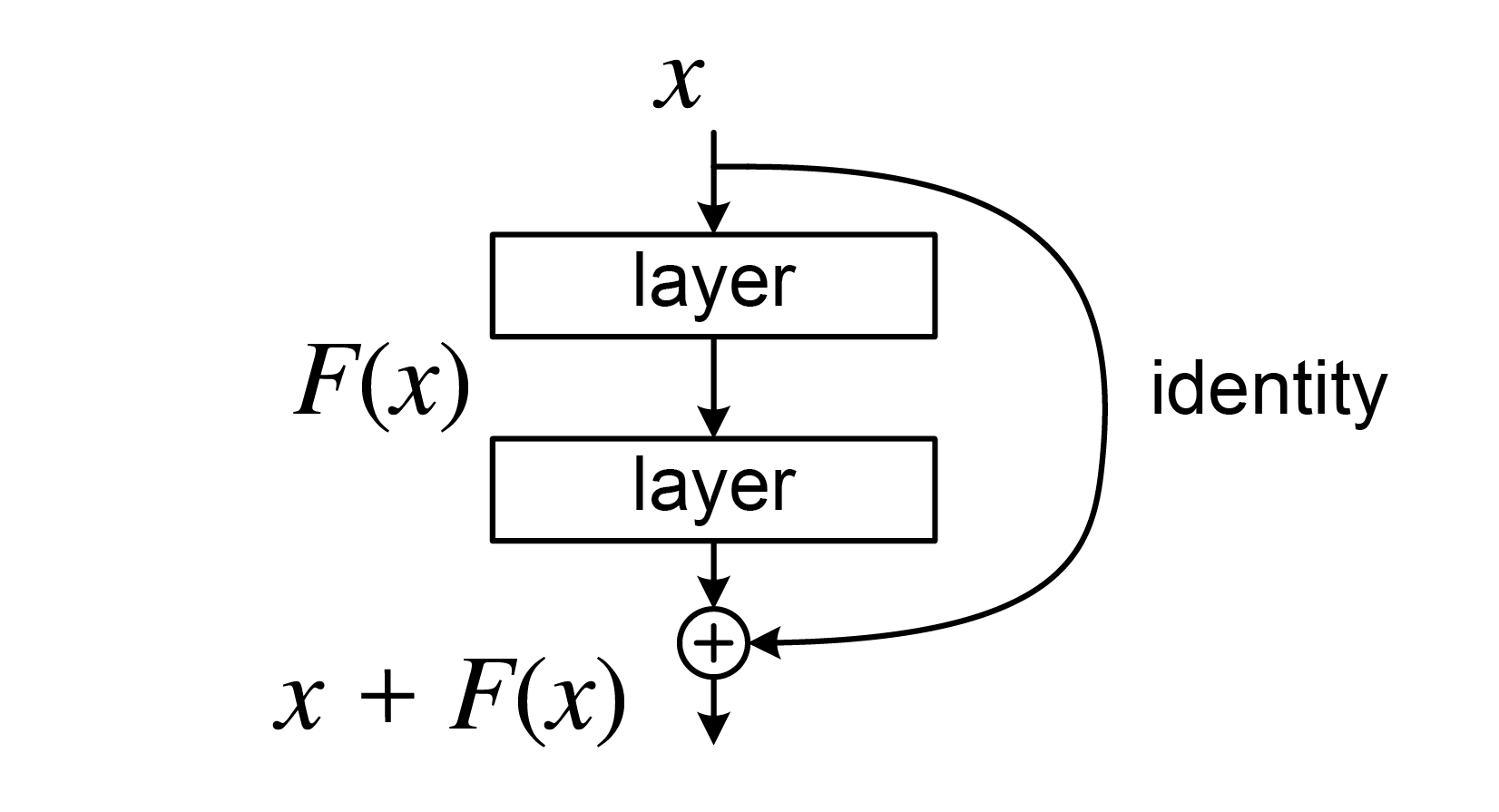
• A residual building block is defined as: $y = F(x, \{W_i\}) + x$
• $x$ and $y$ are the input and output vectors of the layers
• $F(x, \{W_i\})$ represents the residual mapping to be learned
• For a two-layer example: $F = W_2\sigma(W_1x)$, where $\sigma$ is the ReLU activation function

Shortcut Connections

• The operation $F + x$ is performed through a shortcut connection and element-wise addition
• A second nonlinearity is applied after addition: $\sigma(y)$
• Crucially, shortcut connections introduce neither extra parameters nor computational complexity
• This enables fair comparisons between plain and residual networks with identical parameters, depth, width, and computational cost

Dimension Matching

• The dimensions of $x$ and $F(x)$ must be equal for element-wise addition
• When dimensions don't match (e.g., changing input/output channels), a linear projection $W_s$ is used: $y = F(x, \{W_i\}) + W_sx$
• Experiments show that identity mapping is sufficient for addressing degradation and is more economical
• Therefore, $W_s$ is only used when necessary for dimension matching

Flexibility and Applications

• The residual function $F$ is flexible and typically involves two or three layers, though more are possible
• Single-layer residual functions become similar to linear layers and haven't shown advantages
• While notation uses fully-connected layers for simplicity, the concepts apply equally to convolutional layers
• For convolutional layers, element-wise addition is performed on feature maps, channel by channel

Network Architectures

Plain Network Design

• Inspired by VGG nets, using primarily $3 \times 3$ convolutional layers
• Two key design rules:
  • Layers with the same output feature map size have the same number of filters
  • When feature map size is halved, the number of filters is doubled to maintain time complexity per layer
• Downsampling uses convolutional layers with stride 2
• The network ends with global average pooling and a 1000-way fully-connected layer with softmax
• The 34-layer plain network has 3.6 billion FLOPs, which is only 18% of VGG-19's complexity

Residual Network Design

• Built on the plain network by inserting shortcut connections to create residual blocks
• Identity shortcuts are used when input and output dimensions are the same
• Two strategies for dimension matching:
  • Identity mapping with zero-padding for increased dimensions (no extra parameters)
  • Projection shortcuts using $1 \times 1$ convolutions for dimension matching
• The residual architecture maintains the same computational efficiency as the plain network while enabling much deeper networks to be trained effectively