Paper Link

Code

import numpy as np
 
class LSTM:
    def __init__(self, input_size, hidden_size):
        self.input_size = input_size
        self.hidden_size = hidden_size
 
        # Initialize weights and biases
        self.Wf = np.random.randn(hidden_size, input_size + hidden_size)
        self.Wi = np.random.randn(hidden_size, input_size + hidden_size)
        self.Wc = np.random.randn(hidden_size, input_size + hidden_size)
        self.Wo = np.random.randn(hidden_size, input_size + hidden_size)
 
        self.bf = np.zeros((hidden_size, 1))
        self.bi = np.zeros((hidden_size, 1))
        self.bc = np.zeros((hidden_size, 1))
        self.bo = np.zeros((hidden_size, 1))
 
    def sigmoid(self, x):
        return 1 / (1 + np.exp(-x))
 
    def forward(self, x, initial_hidden_state, initial_cell_state):
        h, c = initial_hidden_state.copy(), initial_cell_state.copy()
        hidden_history = []
 
        for t in range(x.shape[0]):
            x_t = x[t].reshape(-1, 1) # (input_size, 1)
            concat = np.vstack((h, x_t)) # (hidden+input, 1)
 
            # Forget gate
            ft = self.sigmoid(np.dot(self.Wf, concat) + self.bf)
 
            # Input gate
            it = self.sigmoid(np.dot(self.Wi, concat) + self.bi)
            
            # Candidate
            c_tilde = np.tanh(np.dot(self.Wc, concat) + self.bc)
 
            # Cell state update
            c = ft * c + it * c_tilde
 
            # Output gate
            ot = self.sigmoid(np.dot(self.Wo, concat) + self.bo)
 
            # Hidden state update
            h = ot * np.tanh(c)
            hidden_history.append(h)
        
        return np.array(hidden_history), h, c

Notes

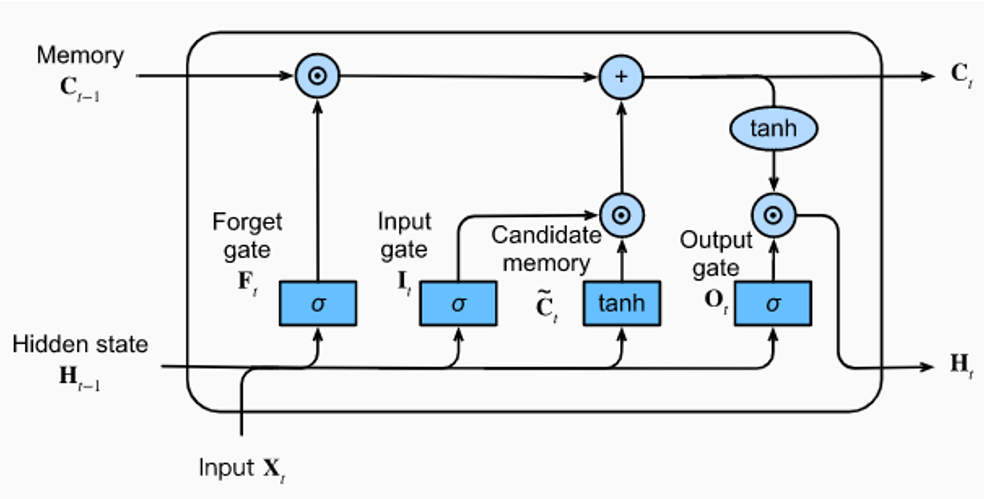
Image Credits: https://medium.com/@ottaviocalzone/an-intuitive-explanation-of-lstm-a035eb6ab42c

• An LSTM unit receives three vectors as input
  • Two vectors (cell state and hidden state) were generated by the LSTM at t - 1
  • The input vector comes from outside and enters the LSTM at t

Understanding the Gates

The LSTM uses three gates to control information flow, each serving a specific purpose in managing the cell's memory.

• Forget Gate: Decides what information from the previous cell state should be discarded.

  • $f_t = \sigma(W_f \cdot [h_{t-1}, x_t] + b_f)$.
  • Output range [0, 1] via sigmoid (1 = keep, 0 = forget).
  • Basically uses the previous hidden state and input vector to decide what to "forget" from the cell state
  • Example: Discards irrelevant information like "the mat" when no longer needed.

• Input Gate: Controls what new information should be added to the cell state in two steps:

  • As seen from $i_t \odot \tilde{C}_t$ , candidate memory proposes new content and input gate decides how much of it to use
  • Decision: What values to update? $i_t = \sigma(W_i \cdot [h_{t-1}, x_t] + b_i)$
  • Candidate: New values to add? $\tilde{C}_t = \tanh(W_C \cdot [h_{t-1}, x_t] + b_C)$ Sigmoid decides which values to update [0,1], tanh creates candidates [-1,1]. Example: Stores information about "the cat eating" when relevant.

• Cell State Update: Actual memory update combining forget and input: $C_t = f_t \odot C_{t-1} + i_t \odot \tilde{C}_t$ where $\odot$ is element-wise multiplication.

  • First term keeps old memory, second adds new info. Additive structure prevents vanishing gradients.

• Output Gate: Decides what parts of cell state to expose as output: $o_t = \sigma(W_o \cdot [h_{t-1}, x_t] + b_o)$, $h_t = o_t \odot \tanh(C_t)$.

  • Applies tanh to cell state [-1,1], then filters output. Example: Exposes only relevant attributes like "hungry" for prediction.

How LSTMs are an improvement over vanilla RNNs

• Vanilla RNN Problem: Traditional RNNs suffer from vanishing/exploding gradients due to multiplicative updates: $h_t = \tanh(W_{hh} h_{t-1} + W_{xh} x_t + b)$

• LSTM Solution: LSTMs use additive cell state updates instead: $C_t = f_t \odot C_{t-1} + i_t \odot \tilde{C}_t$

• Gradient Flow: During backpropagation, gradients flow more easily: $\frac{\partial C_t}{\partial C_{t-1}} = f_t$ Since $f_t \in [0, 1]$, gradients neither vanish nor explode completely, allowing long-term dependencies to be learned.

• Gates Learn Importance: Unlike vanilla RNNs that treat all history equally, LSTM gates learn what information to keep, forget, or emphasize at each timestep.