Playing Atari with Deep Reinforcement Learning
Deep Q-Network (DQN) combines Q-learning with convolutional neural networks to learn control policies directly from raw pixel inputs in Atari games, using experience replay to stabilize training and achieve human-level performance.
Paper Link
Key Definitions
| Term | Definition |
|---|---|
| Q-learning | - Q-learning is a model-free reinforcement learning algorithm used to find the optimal action-selection policy for any given finite Markov decision process (MDP) - The goal of Q-learning is to learn a policy that maximizes the total reward an agent can accumulate over time. |
| Markov Decision Process (MDP) | - A Markov Decision Process (MDP) is a mathematical framework used to describe an environment in reinforcement learning, where an agent interacts with the environment to achieve a goal. - MDPs provide a formalism for modeling decision-making situations where outcomes are partly random and partly under the control of the decision-maker. Components of an MDP: • States (S): A finite set of states that represent all possible situations in the environment. • Actions (A): A finite set of actions available to the agent. • Transition Function (P): A probability function that defines the probability of transitioning to state from state when action is taken. • Reward Function (R): A reward function that specifies the immediate reward received after transitioning to state due to action . • Discount Factor : A factor that discounts future rewards, reflecting the idea that immediate rewards are more valuable than distant rewards. |
| Bellman Equation | - The Bellman equation is a fundamental recursive formula used in dynamic programming and reinforcement learning to determine the optimal policy and value function for a given Markov Decision Process (MDP) - The Bellman equation expresses the idea that the value of a state (or state-action pair) under the optimal policy is equal to the immediate reward plus the discounted value of the next state (or state-action pair), assuming the best possible actions are taken in the future - This recursive relationship allows the value function to be computed iteratively or recursively. |
| Q-network | - A Q-network is a type of neural network used in reinforcement learning to approximate the action-value function, also known as the Q-function • Input Layer: ◦ The input to the Q-network consists of the state representation. In the context of the Atari games discussed in the paper, the input is an 84×84×4 image produced by preprocessing raw frames from the game. This preprocessing includes converting the images to grayscale, resizing, and stacking the last four frames. • Hidden Layers: ◦ The hidden layers are composed of convolutional layers followed by rectified linear units (ReLU) activations. The architecture described in the paper includes: ▪ First Hidden Layer: Convolves 16 filters of size 8×8 with stride 4 with the input image, followed by ReLU. ▪ Second Hidden Layer: Convolves 32 filters of size 4×4 with stride 2, followed by ReLU. ▪ Fully Connected Layer: 256 ReLU units. • Output Layer: ◦ The output layer is a fully connected linear layer with a single output for each possible action. The number of outputs corresponds to the number of valid actions in the game. Each output represents the Q-value for the corresponding action given the input state. |
Introduction
- Context and Motivation
- The paper addresses a key challenge in reinforcement learning (RL): learning control policies directly from high-dimensional sensory inputs, such as vision and speech
- Traditional RL applications in these domains have relied on hand-crafted features combined with linear value functions or policy representations
- The effectiveness of such systems heavily depends on the quality of the feature representation used
- The application of deep learning techniques to RL poses several challenges
- Sparse and Delayed Rewards: Unlike supervised learning, which typically requires large amounts of hand-labeled data, RL algorithms must learn from scalar reward signals that are often sparse, noisy, and delayed
- Correlated States: RL often deals with sequences of highly correlated states, contrary to the assumption of independence in most deep learning algorithms
- Non-stationary Data Distribution: The data distribution in RL changes as the agent learns new behaviors, complicating the learning process for deep learning methods that generally assume a fixed underlying distribution
Key Contributions of the Paper
- The paper demonstrates that a convolutional neural network (CNN) can overcome these challenges to learn successful control policies from raw video data in complex RL environments
- The network is trained using a variant of the Q-learning algorithm, with stochastic gradient descent used to update the weights
- To address the issues of correlated data and non-stationary distributions, the authors use an experience replay mechanism, which randomly samples previous transitions and thus smooths the training distribution over many past behaviors
Key Results
- Generalization
- The goal was to create a single neural network agent capable of playing multiple games without any game-specific information or hand-designed visual features
- The agent learned solely from video input, reward signals, and terminal signals, mimicking a human player's experience
- Performance
- The network architecture and all hyperparameters were kept constant across the games
- The network outperformed all previous RL algorithms on six of the seven games tested and surpassed expert human players on three of them
Background
- The section describes how an agent interacts with an environment in a sequence of actions, observations, and rewards
- Specifically, the environment considered is the Atari emulator, where the agent selects an action from the set of legal game actions at each time step
- Elements of the Environment
- Actions (A): The set of all possible actions the agent can take
- State (s): At each time step, the agent observes an image from the emulator, which is a vector of raw pixel values representing the current screen
- Rewards (r): The agent receives a reward representing the change in the game score after each action
- Since the agent only observes the current screen image, the task is partially observed
- Many states of the emulator can be perceptually aliased, meaning that different states might look the same to the agent
- Therefore, the agent considers sequences of actions and observations to learn effective strategies
- The interaction between the agent and the environment is formalized as a large but finite Markov Decision Process (MDP), where each sequence of actions and observations is considered a distinct state
- The goal of the agent is to maximize the future rewards by interacting with the emulator and selecting actions strategically
- Future rewards are discounted by a factor per time step, which means immediate rewards are valued higher than distant rewards
- The optimal action-value function is defined as the maximum expected return achievable by following any strategy after seeing some sequence and taking action
- This function obeys an important identity known as the Bellman equation: where is the next state after taking action from state
- Many reinforcement learning algorithms estimate the action-value function using the Bellman equation as an iterative update
- These algorithms converge to the optimal action-value function over time
- In practice, instead of estimating the action-value function separately for each sequence, a function approximator is used
- This can be a linear function approximator or a neural network, known as a Q-network
- The Q-network is trained by minimizing a sequence of loss functions, with updates performed using stochastic gradient descent
Deep Reinforcement Learning
- A key innovation is combining Q-learning with deep neural networks, referred to as Deep Q-Learning
- This approach involves using a convolutional neural network (CNN) to approximate the Q-function, which estimates the expected cumulative reward for each action given the current state
- To address the challenges of correlated data and non-stationary distributions in reinforcement learning, the authors use an experience replay mechanism
- Experience replay involves storing the agent's experiences at each time-step in a replay memory and sampling mini-batches of experiences to update the Q-network
- This technique helps to smooth out learning and reduce the variance of updates, making the training process more stable
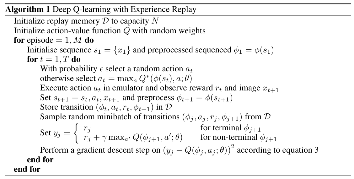
Algorithm Walkthrough
-
Initialization
- Create a replay memory D with capacity N (e.g., 1 million transitions)
- Initialize Q-network with random weights θ
- Prepare initial state by preprocessing and stacking frames
-
For each episode (game)
- Initialize Episode
- Reset the game
- Preprocess the first frame and stack it 4 times to create initial state
- For each timestep t in the episode
- Action Selection (ε-greedy policy)
- With probability ε: select random action (exploration)
- With probability (1-ε): select action (exploitation)
- Execute Action
- Perform action a in the emulator
- Observe reward r and next raw frame
- Preprocess new frame and append to create next state
- Store Transition
- Save transition in replay memory D
- If memory is full, remove oldest transition
- Sample and Learn
- Randomly sample mini-batch of transitions from D (e.g., 32 transitions)
- For each transition in mini-batch:
- If episode terminated: target
- If episode continues: target
- Perform gradient descent step on loss:
- Update State
- Set for next iteration
- Repeat until episode terminates
- Action Selection (ε-greedy policy)
- Initialize Episode
-
Advantages of Experience Replay:
- Data Efficiency: Each step of experience is potentially used in multiple updates, improving data efficiency.
- Reduced Correlation: Randomizing the samples breaks the strong correlations between consecutive experiences.
- Stabilized Learning: Averaging over many previous states smooths out the learning process and prevents oscillations or divergence in the Q-network parameters.
Demo: DQN replay playground
DQN replay playground
A tiny 1D world shows epsilon-greedy action choice, experience replay, and Bellman targets updating a small Q-table.
Replay buffer
No transitions yet. Take a step.
Q-table
Latest Bellman update
No update yet.
This demo simulates a simplified reinforcement learning agent learning to navigate a 1D world. The agent starts in the middle (S2) and can move left or right. The goal is to reach S4 (Win, +1 reward) while avoiding S0 (Lose, -1 reward).
What's happening:
- Each step, the agent selects an action using epsilon-greedy policy, moves in the world, and stores the experience in a replay buffer
- The Q-table shows the estimated value of each action in each state (higher values = better)
- The replay buffer stores past transitions, and the agent learns by randomly sampling batches from this buffer
- Q-values are updated using the Bellman equation:
Parameter controls:
- Epsilon (explore): Controls the exploration-exploitation tradeoff. Higher values (closer to 1.0) mean more random exploration, lower values (closer to 0.0) mean the agent follows its learned Q-values more. Start high to explore, then decrease over time.
- Gamma (discount): How much the agent values future rewards vs. immediate rewards. Higher values (closer to 1.0) make the agent plan further ahead, lower values make it focus on immediate rewards.
- Alpha (learning rate): How quickly the Q-values update. Higher values mean faster learning but can be unstable, lower values are more stable but learn slower.
- Replay batch size: Number of past experiences sampled from the buffer for each update. Larger batches provide more stable updates but use more memory.
- Replay capacity: Maximum number of transitions stored in the replay buffer. Larger buffers store more diverse experiences but use more memory.
Try clicking "Step ×5" a few times and watch the Q-values update. Notice how the agent learns that moving right from S3 is valuable (leads to Win), and this knowledge propagates backward through the states.
Code
import random
from collections import deque
import numpy as np

def epsilon_greedy(q, state, epsilon):
    if random.random() < epsilon:
        return random.randrange(q.shape[1])
    return int(np.argmax(q[state]))

def bellman_target(q, reward, next_state, done, gamma):
    if done:
        return reward
    return reward + gamma * np.max(q[next_state])

def train_step(q, buffer, batch_size, gamma, alpha):
    batch = random.sample(buffer, min(batch_size, len(buffer)))
    for (s, a, r, s2, done) in batch:
        target = bellman_target(q, r, s2, done, gamma)
        q[s, a] += alpha * (target - q[s, a])

q = np.zeros((num_states, num_actions))
buffer = deque(maxlen=1000)

state = env.reset()
for t in range(steps):
    action = epsilon_greedy(q, state, epsilon)
    next_state, reward, done = env.step(action)
    buffer.append((state, action, reward, next_state, done))
    train_step(q, buffer, batch_size=32, gamma=0.99, alpha=0.1)
    state = env.reset() if done else next_state
Model Architecture
- Input Layer
- Input to the neural network is an 84x84x4 image produced by stacking four preprocessed frames
- First Convolutional layer applies 16 filters of size 8x8 with stride 4
- Second Conv layer applies 32 filters of size 4x4 with stride 2
- Third Conv layer 64 filters of 3x3 with stride 1
- Proceeded by Fully Connected Layer, and the output layer has a single output for each valid action in the game, representing the Q-values for the respective actions
- Purpose
- The convolutional layers serve to automatically extract high-level spatial and temporal features from the raw pixel data
- The fully connected layers combine the extracted features to compute the Q-values for each action
- The Q-values represent the expected cumulative rewards for taking each action in the given state, guiding the agent's decision-making process
Evaluation Criteria
- Average Total Reward
- The main evaluation metric was the average total reward the agent accumulated in an episode or game.
- Periodic evaluations were conducted during training by running an epsilon-greedy policy with epsilon set to 0.05.
- Policy’s Estimated Action-Value Function (Q)
- In addition to the total reward, the authors tracked the policy’s estimated action-value function, which provided an estimate of the expected discounted reward for following the policy from any given state.
- This metric was more stable than the total reward and provided insight into the learning progress of the agent.